Adaptive Asset Allocation Extended
This post extends the replication from the Adaptive Asset Allocation Replication post by running the analysis on OOS (out-of-sample) data from 2015 through 2023. Thanks to Dale Rosenthal for helpful comments.
The paper uses the 5 portfolios below. Each section of this post will give a short description of the portfolio construction and then focus on comparing the OOS results with the replicated and original results. See the other post for details on the data and portfolio construction methodologies.
- Equal weight of all asset classes
- Equal risk contribution of all asset classes
- Equal weight of highest momentum asset classes
- Equal risk contribution of highest momentum asset classes
- Minimum variance of highest momentum asset classes
The table below summarizes the date ranges for each sample period in this post.
| Period | Date Range |
|---|---|
| Replication | Feb 1996 - Dec 2014 |
| OOS | Jan 2015 - Dec 2023 |
| 2015-2021 | Jan 2015 - Dec 2021 |
| Full | Feb 1996 - Dec 2023 |
This post uses the ftblog package. You can install it using the remotes::install_github() function in the code block below. First we need to setup our environment with the necessary packages, data, and functions.
# remotes::install_github("joshuaulrich/ftblog")
suppressPackageStartupMessages({
    library(ftblog)
    library(PerformanceAnalytics)
})

data(aaa_returns, package = "ftblog")
returns <- aaa_returns[, -1]    # no cash
r_rep   <- returns["/2014"]
r_oos   <- returns["2014-07/"]  # need 6 months for 120-day lags (this is 128 days)
r_full  <- returns

# calculate strategy statistics
strat_summary <-
function(returns,
         original_results = NULL)
{
    stats <- table.AnnualizedReturns(returns)
    stats <- rbind(stats,
                   "Worst Drawdown" = -maxDrawdown(returns))

    if (!is.null(original_results)) {
        stats <- cbind(original_results, stats)
        colnames(stats)[1] <- "Original"
    }

    stats <- round(stats, 3)

    return(stats)
}

chart_performance <-
function(R,
         title = "Performance")
{
    stopifnot(all(c("Replication", "OOS") %in% colnames(R)))
    r <- R[, c("Replication", "OOS")]
    p <- chart.CumReturns(r,
                          main = title,
                          main.timespan = FALSE,
                          yaxis.right = TRUE)
    p <- addLegend("topleft", lty = 1, lwd = 1)
    p <- addSeries(r[,1], type = "h", main = "Return")
    p <- addSeries(r[,2], type = "h", on = 0, col = "red")
    p <- addSeries(Drawdowns(r), main = "Drawdown")
    p
}
1. Equal weight portfolio of all asset classes
This portfolio assumes no knowledge of expected relative asset class performance, risk, or correlation. It holds each asset class in equal weight and is rebalanced monthly.
rr_equal_weight <- as.xts(apply(returns["/2014"], 1, mean))
ro_equal_weight <- as.xts(apply(returns["2015/"], 1, mean))
rf_equal_weight <- as.xts(apply(returns, 1, mean))

monthly_returns <-
  merge(Replication = to_monthly_returns(rr_equal_weight),
        OOS = to_monthly_returns(ro_equal_weight),
        "2015-2021" = to_monthly_returns(ro_equal_weight["2015/2021"]),
        Full = to_monthly_returns(rf_equal_weight),
        check.names = FALSE)

stats <- strat_summary(monthly_returns)
chart_performance(monthly_returns, "All Assets - Equal Weight")
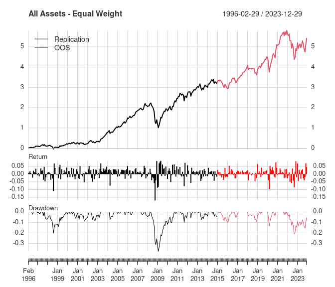
| Replication | OOS | 2015-2021 | Full | |
|---|---|---|---|---|
| Annualized Return | 0.079 | 0.049 | 0.072 | 0.069 |
| Annualized Std Dev | 0.115 | 0.107 | 0.091 | 0.112 |
| Annualized Sharpe (Rf=0%) | 0.684 | 0.456 | 0.794 | 0.614 |
| Worst Drawdown | -0.377 | -0.210 | -0.136 | -0.377 |
The OOS annualized return is significantly less than the prior results. This is largely due to the -21.0% drawdown that started in 2022 and is still ongoing. Note that the full-period results are very similar to the replication results, though the 2022 drawdown did decrease the annualized return by ~1%.
Note that this portfolio’s results from 2015-2021 are very similar to the replication results through the end of 2014. That suggests the 2022 bear market is the main cause for the lower return in the OOS results.
2. Equal risk contribution using all asset classes
The next portfolio assumes the investor has some knowledge of each asset’s risk, but still no knowledge of relative performance or correlations. So each asset in this portfolio is given a weight proportional to its historical relative risk, with the hope that each asset will contribute the same amount of risk to the overall portfolio in the future.
rr_equal_risk <- portf_return_equal_risk(r_rep, 120, 60)
ro_equal_risk <- portf_return_equal_risk(r_oos, 120, 60)
rf_equal_risk <- portf_return_equal_risk(r_full, 120, 60)

monthly_returns <-
  merge(to_monthly_returns(rr_equal_risk),
        to_monthly_returns(ro_equal_risk["2015/"]),
        to_monthly_returns(ro_equal_risk["2015/2021"]),
        to_monthly_returns(rf_equal_risk))
colnames(monthly_returns) <- c("Replication", "OOS", "2015-2021", "Full")

stats <- strat_summary(monthly_returns)
chart_performance(monthly_returns, "All Assets - Equal Risk")

| Replication | OOS | 2015-2021 | Full | |
|---|---|---|---|---|
| Annualized Return | 0.086 | 0.034 | 0.056 | 0.069 |
| Annualized Std Dev | 0.073 | 0.082 | 0.061 | 0.076 |
| Annualized Sharpe (Rf=0%) | 1.177 | 0.411 | 0.908 | 0.903 |
| Worst Drawdown | -0.142 | -0.194 | -0.071 | -0.194 |
Like the equal weight portfolio, this portfolio’s OOS annualized return is significantly lower than the replication results. This methodology only slightly reduced the 2022 drawdown to -19.4% from -21.0%. The maximum drawdown is now in 2022 instead of during the 2008 financial crisis.
In the replication, the equal risk contribution portfolio results are better than the equal weight portfolio, but the OOS equal risk portfolio did not show similar improvement. Even when 2022 is excluded, the OOS equal risk portfolio didn’t show improvement over the equal weight portfolio.
3. Equal weight portfolio of highest momentum asset classes
The next portfolio assumes the investor has some knowledge of each asset’s returns, but still no knowledge of risk or correlations. Asset returns are based on 6-month momentum (approximately 120 days). Momentum is re-estimated every month and only the top 5 assets are included in the portfolio.
rr_momo_eq_wt <- portf_return_momo(r_rep, 5, 120)
ro_momo_eq_wt <- portf_return_momo(r_oos, 5, 120)
rf_momo_eq_wt <- portf_return_momo(r_full, 5, 120)

monthly_returns <-
  merge(to_monthly_returns(rr_momo_eq_wt),
        to_monthly_returns(ro_momo_eq_wt["2015/"]),
        to_monthly_returns(ro_momo_eq_wt["2015/2021"]),
        to_monthly_returns(rf_momo_eq_wt))
colnames(monthly_returns) <- c("Replication", "OOS", "2015-2021", "Full")

stats <- strat_summary(monthly_returns)
chart_performance(monthly_returns, "Top 5 Momentum Assets - Equal Weight")
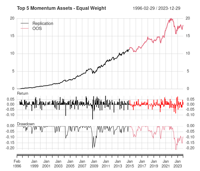
| Replication | OOS | 2015-2021 | Full | |
|---|---|---|---|---|
| Annualized Return | 0.142 | 0.051 | 0.081 | 0.112 |
| Annualized Std Dev | 0.114 | 0.104 | 0.092 | 0.111 |
| Annualized Sharpe (Rf=0%) | 1.243 | 0.488 | 0.884 | 1.001 |
| Worst Drawdown | -0.199 | -0.213 | -0.114 | -0.213 |
Again, the OOS annualized return is significantly worse than the replicated results. The OOS results for this portfolio show improvement in the Sharpe Ratio versus the equal risk contribution portfolio (2). The replicated results for this portfolio showed similar improvements versus portfolio (2).
In the replication, equal weight momentum results are better than the equal risk portfolio. But the OOS equal weight momentum portfolio did not show significant improvement versus the equal risk portfolio (2), and is roughly the same as the equal weight portfolio (1).
4. Equal risk contribution portfolio of highest momentum asset classes
The previous two portfolios estimated asset weights using either risk-based or momentum-based weights. This next portfolio combines estimates of momentum-based performance and accounts for asset class risk differences. It includes the top 5 asset classes based on 6-month returns and weights them using the same equal risk contribution method as portfolio (2).
rr_momo_eq_risk <- portf_return_momo_equal_risk(r_rep, 5, 120, 60)
ro_momo_eq_risk <- portf_return_momo_equal_risk(r_oos, 5, 120, 60)
rf_momo_eq_risk <- portf_return_momo_equal_risk(r_full, 5, 120, 60)

monthly_returns <-
  merge(to_monthly_returns(rr_momo_eq_risk),
        to_monthly_returns(ro_momo_eq_risk["2015/"]),
        to_monthly_returns(ro_momo_eq_risk["2015/2021"]),
        to_monthly_returns(rf_momo_eq_risk))
colnames(monthly_returns) <- c("Replication", "OOS", "2015-2021", "Full")

stats <- strat_summary(monthly_returns)
chart_performance(monthly_returns, "Top 5 Momentum Assets - Equal Risk")
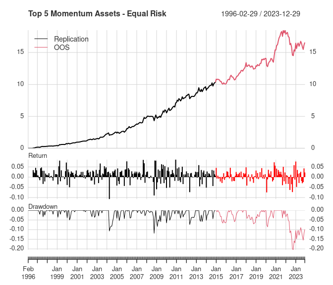
| Replication | OOS | 2015-2021 | Full | |
|---|---|---|---|---|
| Annualized Return | 0.137 | 0.050 | 0.081 | 0.108 |
| Annualized Std Dev | 0.102 | 0.095 | 0.081 | 0.100 |
| Annualized Sharpe (Rf=0%) | 1.335 | 0.528 | 0.991 | 1.076 |
| Worst Drawdown | -0.119 | -0.204 | -0.086 | -0.204 |
It’s clear that the major cause of the poorer OOS performance of this portfolio is due to how it handled the 2022 bear market. This portfolio handled the 2008 financial crisis very well, but it offered almost no protection in 2022. This indicates there was a fundamental difference in 2008 versus 2022 in the asset classes held by this portfolio.
Similar to the replicated results, the reduction in risk is the main benefit of this portfolio versus the equal weight momentum portfolio (3). That said, the OOS performance of this portfolio only showed marginal improvement versus portfolio (3). Even more notable, this portfolio didn’t improve returns versus the simple equal weight portfolio (1) during the OOS period like it did for the replication period.
5. Minimum variance portfolio of highest momentum asset classes
The final portfolio takes the above concepts and adds correlation estimates to the portfolio optimization. The previous portfolios only accounted for the relative risk between the asset classes, but not the correlation between the assets’ returns. This portfolio accounts for the correlations between asset classes by finding the minimum variance portfolio.
rr_momo_min_var <- portf_return_momo_min_var(r_rep, 5, 120, 60, "above average")
ro_momo_min_var <- portf_return_momo_min_var(r_oos, 5, 120, 60, "above average")
rf_momo_min_var <- portf_return_momo_min_var(r_full, 5, 120, 60, "above average")

monthly_returns <-
  merge(to_monthly_returns(rr_momo_min_var),
        to_monthly_returns(ro_momo_min_var["2015/"]),
        to_monthly_returns(ro_momo_min_var["2015/2021"]),
        to_monthly_returns(rf_momo_min_var))
colnames(monthly_returns) <- c("Replication", "OOS", "2015-2021", "Full")

stats <- strat_summary(monthly_returns)
chart_performance(monthly_returns, "Above Average 6mo Momentum - Min Var")
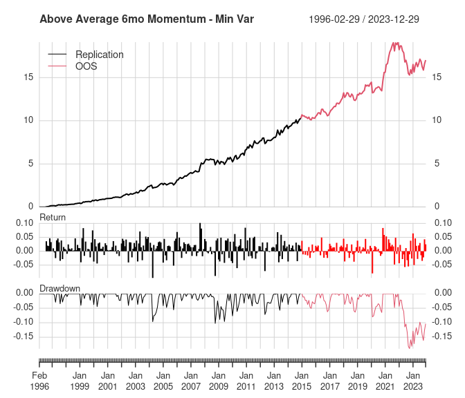
| Replication | OOS | 2015-2021 | Full | |
|---|---|---|---|---|
| Annualized Return | 0.130 | 0.058 | 0.082 | 0.106 |
| Annualized Std Dev | 0.099 | 0.095 | 0.081 | 0.098 |
| Annualized Sharpe (Rf=0%) | 1.315 | 0.612 | 1.008 | 1.086 |
| Worst Drawdown | -0.112 | -0.162 | -0.083 | -0.162 |
Recall that the original results for portfolio (5) showed improved return and lower maximum drawdown versus portfolio (4), while the replicated results were almost the same for both portfolios. The OOS results for these two portfolios are also very similar. In the 2015-2021 period, portfolio (5) has a slightly higher return and Sharpe ratio and lower max drawdown than portfolio (4).
Conclusion
For all 5 portfolios, the OOS results are not as good as the replicated results. This is largely due to the 2022 bear market, but the 2015-2021 results still aren’t as good as the replicated results.
Allocate Smartly has a great post about 2022 bear market performance of tactical asset allocation (TAA) strategies like this one. They find that TAA strategies did poorly in the 2022 bear market if they assumed intermediate and long-term bonds provide diversification from risky assets. Both risk assets and longer duration bonds performed poorly in 2022, and the correlation between bonds and equities was positive instead of negative like they have been historically.
In a future post, I may investigate how these portfolios would have performed if they were allowed to allocate to short-term Treasuries.
Portfolio Results by Sample Period
This section contains tables with results for all portfolios in a particular sample period.
Replication Period
| Equal Weight | Equal Risk | Momo Eq Weight | Momo Eq Risk | Momo Min Var | |
|---|---|---|---|---|---|
| Ann. Return | 0.079 | 0.086 | 0.142 | 0.137 | 0.130 |
| Ann. Std Dev | 0.115 | 0.073 | 0.114 | 0.102 | 0.099 |
| Ann. Sharpe | 0.684 | 1.177 | 1.243 | 1.335 | 1.315 |
| Max Drawdown | -0.377 | -0.142 | -0.199 | -0.119 | -0.112 |
Out-of-Sample: 2015-2023
| Equal Weight | Equal Risk | Momo Eq Weight | Momo Eq Risk | Momo Min Var | |
|---|---|---|---|---|---|
| Ann. Return | 0.049 | 0.034 | 0.051 | 0.050 | 0.058 |
| Ann. Std Dev | 0.107 | 0.082 | 0.104 | 0.095 | 0.095 |
| Ann. Sharpe | 0.456 | 0.411 | 0.488 | 0.528 | 0.612 |
| Max Drawdown | -0.210 | -0.194 | -0.213 | -0.204 | -0.162 |
Out-of-Sample: 2015-2021
| Equal Weight | Equal Risk | Momo Eq Weight | Momo Eq Risk | Momo Min Var | |
|---|---|---|---|---|---|
| Ann. Return | 0.072 | 0.056 | 0.081 | 0.081 | 0.082 |
| Ann. Std Dev | 0.091 | 0.061 | 0.092 | 0.081 | 0.081 |
| Ann. Sharpe | 0.794 | 0.908 | 0.884 | 0.991 | 1.008 |
| Max Drawdown | -0.136 | -0.071 | -0.114 | -0.086 | -0.083 |
If you love using my open-source work (e.g. quantmod, TTR, xts, IBrokers, microbenchmark, blotter, quantstrat, etc.), you can give back by sponsoring me on GitHub. I truly appreciate anything you’re willing and able to give!