Historical / Future Volatility Correlation Stability
Michael Stokes, author of the MarketSci blog recently published a thought-provoking post about the correlation between historical and future volatility (measured as the standard deviation of daily close price percentage changes). This post is intended as an extension of his “unfinished thought”, not a critique.
He suggests using his table of volatility correlations as a back-of-the-envelope approach to estimate future volatility, which led me to question the stability of the correlations in his table. His table’s values are calculated using daily data from 1970-present… but what if you were to calculate correlations using only one year of data, rather than thirty? The chart below shows the results.
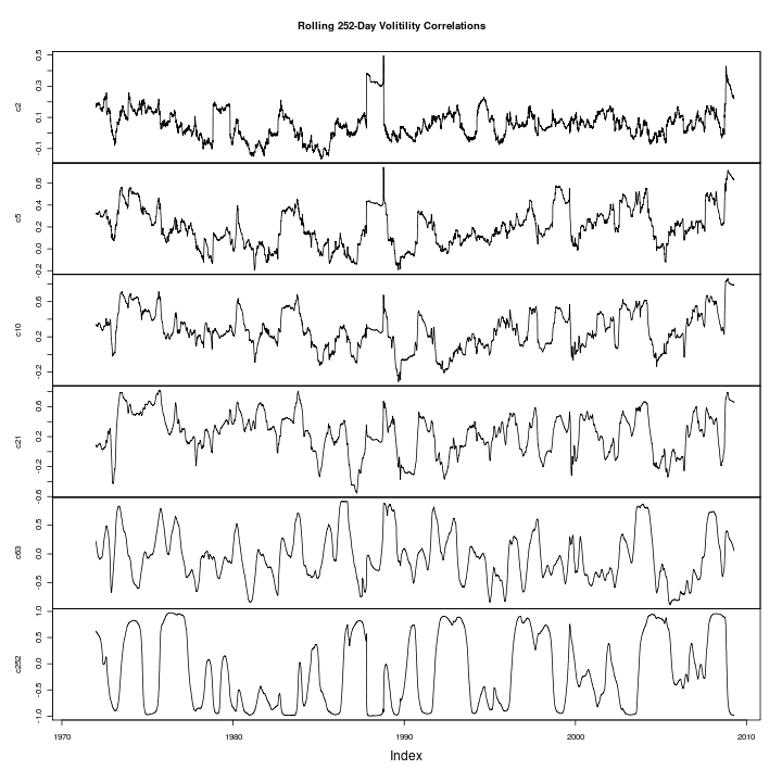
The chart shows the rolling one-year (252-day) correlations for the diagonal in Michael’s table (e.g. historical and future 2-day volatility, …, historical and future 252-day volatility). You can see the shorter periods are generally more stable, but are also closer to zero. The rolling one-year correlation between historical and future one-year volatility swings wildly from +/-1 over time.
This isn’t to argue that Michael’s back-of-the-envelope approach is incorrect, rather it is an attempt to make the approach more robust by weighing long-term market characteristics against recent market behavior.
For those interested, here is the R code I used to replicate Michael’s table and create the graph above. An interesting extension of this analysis would be to calculate volatility using TTR’s volatility() function instead of standard deviation. I’ll leave that exercise to the interested reader.
require(quantmod)

# pull SPX data from Yahoo Finance
getSymbols("^GSPC",from="1970-01-01")

# volatility horizons
GSPC$v2 <- runSD(ROC(Cl(GSPC)),2)
GSPC$v5 <- runSD(ROC(Cl(GSPC)),5)
GSPC$v10 <- runSD(ROC(Cl(GSPC)),10)
GSPC$v21 <- runSD(ROC(Cl(GSPC)),21)
GSPC$v63 <- runSD(ROC(Cl(GSPC)),63)
GSPC$v252 <- runSD(ROC(Cl(GSPC)),252)

# volatility horizon lags
GSPC$l2 <- lag(GSPC$v2,-2)
GSPC$l5 <- lag(GSPC$v5,-5)
GSPC$l10 <- lag(GSPC$v10,-10)
GSPC$l21 <- lag(GSPC$v21,-21)
GSPC$l63 <- lag(GSPC$v63,-63)
GSPC$l252 <- lag(GSPC$v252,-252)

# volatility correlation table
cor(GSPC[,7:18],use="pair")[1:6,7:12]

# remove missing observations
GSPC <- na.omit(GSPC)

# rolling 1-year volatility correlations
GSPC$c2 <- runCor(GSPC$v2,GSPC$l2,252)
GSPC$c5 <- runCor(GSPC$v5,GSPC$l5,252)
GSPC$c10 <- runCor(GSPC$v10,GSPC$l10,252)
GSPC$c21 <- runCor(GSPC$v21,GSPC$l21,252)
GSPC$c63 <- runCor(GSPC$v63,GSPC$l63,252)
GSPC$c252 <- runCor(GSPC$v252,GSPC$l252,252)

# plot rolling 1-year volatility correlations
plot.zoo(GSPC[,grep("c",colnames(GSPC))],n=1,
  main="Rolling 252-Day Volitility Correlations")
If you love using my open-source work (e.g. quantmod, TTR, xts, IBrokers, microbenchmark, blotter, quantstrat, etc.), you can give back by sponsoring me on GitHub. I truly appreciate anything you’re willing and able to give!