RSI(2) Evaluation
This post continues the series of investigating the RSI(2) strategy. The first post replicated this simple RSI(2) strategy from the MarketSci Blog using R. The second post showed how to replicate the strategy that scales in/out of RSI(2).
If you like the RSI(2), be sure to check out David Varadi’s RSI(2) alternative!
This post will use the PerformanceAnalytics package to evaluate the rules that scale in/out of positions. I’ve also provided a simple function that provides some summary statistics. There is a lot of code, so I put it at the end of the post.
Table 1 contains output from my simple trade summary function (the wins and losses are in percentages, i.e. 0.69 is 69 basis points). The short side of the rule traded more often and had a lower win rate. The short side overcame its lower win rate via much higher mean and median win/loss ratios.
Table 1: RSI(2) Trade Statistics - RSI steps = 5, Size steps = 0.25
| Signal | # Trades | % Win | Mean Win | Mean Loss | Median Win | Median Loss | Mean W/L | Median W/L |
|---|---|---|---|---|---|---|---|---|
| -1.00 | 133 | 58 | 0.69 | -0.44 | 0.53 | -0.25 | 1.55 | 2.12 |
| -0.75 | 173 | 49 | 0.62 | -0.39 | 0.37 | -0.25 | 1.60 | 1.48 |
| -0.50 | 143 | 54 | 0.43 | -0.36 | 0.28 | -0.19 | 1.19 | 1.51 |
| -0.25 | 158 | 56 | 0.21 | -0.19 | 0.14 | -0.13 | 1.15 | 1.08 |
| 0.00 | 1262 | 0 | NaN | NaN | NA | NA | NaN | NA |
| 0.25 | 117 | 53 | 0.26 | -0.31 | 0.18 | -0.21 | 0.83 | 0.86 |
| 0.50 | 137 | 58 | 0.51 | -0.58 | 0.31 | -0.35 | 0.87 | 0.89 |
| 0.75 | 143 | 62 | 0.88 | -0.89 | 0.50 | -0.71 | 0.99 | 0.70 |
| 1.00 | 119 | 63 | 1.34 | -1.41 | 0.80 | -1.11 | 0.95 | 0.71 |
Table 2 shows the output from the PerformanceAnalytics table.Drawdowns() function. The largest percentage drawdown occurred in late 2008, but only lasted a few weeks.
The table also shows the system is prone to drawdowns that trough quickly and take months to recover from. A week of bad trades can take months to recover from.
Table 2: RSI(2) Drawdowns - RSI steps = 5, Size steps = 0.25
| From | Trough | To | Depth | Length | To Trough | Recovery |
|---|---|---|---|---|---|---|
| 2008-10-06 | 2008-10-10 | 2008-10-28 | -0.157 | 17 | 5 | 12 |
| 2001-08-30 | 2001-09-21 | 2002-01-23 | -0.091 | 96 | 12 | 84 |
| 2002-07-19 | 2002-07-23 | 2002-08-20 | -0.088 | 23 | 3 | 20 |
| 2000-03-22 | 2000-04-14 | 2000-07-05 | -0.076 | 73 | 18 | 55 |
| 2009-02-17 | 2009-02-23 | 2009-04-27 | -0.070 | 49 | 5 | 44 |
| 2003-03-14 | 2003-03-21 | 2003-05-09 | -0.055 | 40 | 6 | 34 |
| 2000-10-09 | 2000-10-12 | 2000-12-06 | -0.052 | 42 | 4 | 38 |
| 2002-08-29 | 2002-09-24 | 2002-10-10 | -0.051 | 30 | 18 | 12 |
| 2008-01-02 | 2008-01-22 | 2008-03-11 | -0.045 | 48 | 14 | 34 |
| 2001-04-18 | 2001-06-18 | 2001-08-10 | -0.045 | 81 | 43 | 38 |
Table 3 shows the output from the PerformanceAnalytics table.DownsideRisk() function. The ratio of gain/loss deviation is encouraging. I have to defer to the PerformanceAnalytics documentation and vignettes to describe the rest of the table.
Table 3: RSI(2) Downside Risk - RSI steps = 5, Size steps = 0.25
| Statistic | Return |
|---|---|
| Semi Deviation | 0.0050 |
| Gain Deviation | 0.0094 |
| Loss Deviation | 0.0076 |
| Downside Deviation (MAR=10%) | 0.0099 |
| Downside Deviation (rf=0%) | 0.0092 |
| Downside Deviation (0%) | 0.0092 |
| Maximum Drawdown | -0.1572 |
| VaR (99%) | 0.0160 |
| Beyond VaR | 0.0160 |
| Modified VaR (99%) | 0.0705 |
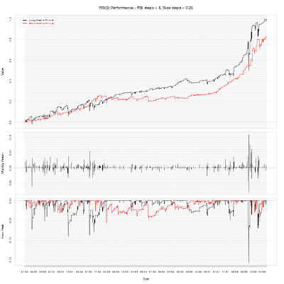
The chart below shows the output from the PerformanceAnalytics charts.PerformanceSummary() function. It shows the equity curves and drawdown from peak for the long and short sides of the strategy. The middle graph shows the daily returns for the combined strategy.
The code below has everything that created the results above. It also contains the same results for a modified RSI(2) strategy. The modified strategy uses RSI steps of 10 and sizing steps of 0.3 (i.e. RSI<10 -> size=1, 10<20 -> size=0.7, etc.).
# Attach packages. You can install packages via:
# install.packages(c("quantmod","TTR","PerformanceAnalytics"))
library(quantmod)
library(TTR)
library(PerformanceAnalytics)

# Pull S&P500 index data from Yahoo! Finance
getSymbols("^GSPC", from="2000-01-01")

# Calculate the RSI indicator
rsi <- RSI(Cl(GSPC), 2)

# Calculate Close-to-Close returns
ret <- ROC(Cl(GSPC))
ret[1] <- 0

# This function gives us some standard summary
# statistics for our trades.
tradeStats <- function(signals, returns) {
# Inputs:
# signals : trading signals
# returns : returns corresponding to signals

# Combine data and convert to data.frame
sysRet <- signals * returns * 100
posRet <- sysRet > 0 # Positive rule returns
negRet <- sysRet < 0 # Negative rule returns
dat <- cbind(signals,posRet*100,sysRet[posRet],sysRet[negRet],1)
dat <- as.data.frame(dat)

# Aggreate data for summary statistics
means <- aggregate(dat[,2:4], by=list(dat[,1]), mean, na.rm=TRUE)
medians <- aggregate(dat[,3:4], by=list(dat[,1]), median, na.rm=TRUE)
sums <- aggregate(dat[,5], by=list(dat[,1]), sum)

colnames(means) <- c("Signal","% Win","Mean Win","Mean Loss")
colnames(medians) <- c("Signal","Median Win","Median Loss")
colnames(sums) <- c("Signal","# Trades")

all <- merge(sums,means)
all <- merge(all,medians)

wl <- cbind( abs(all[,"Mean Win"]/all[,"Mean Loss"]),
abs(all[,"Median Win"]/all[,"Median Loss"]) )
colnames(wl) <- c("Mean W/L","Median W/L")

all <- cbind(all,wl)
return(all)
}

# This function determines position size and
# enables us to test several ideas with much
# greater speed and flexibility.
rsi2pos <- function(ind, indIncr=5, posIncr=0.25) {
# Inputs:
# ind : indicator vector
# indIncr : indicator value increments/breakpoints
# posIncr : position value increments/breakpoints

# Initialize result vector
size <- rep(0,NROW(ind))

# Long
size <- ifelse(ind < 4*indIncr, (1-posIncr*3), size)
size <- ifelse(ind < 3*indIncr, (1-posIncr*2), size)
size <- ifelse(ind < 2*indIncr, (1-posIncr*1), size)
size <- ifelse(ind < 1*indIncr, (1-posIncr*0), size)

# Short
size <- ifelse(ind > 100-4*indIncr, 3*posIncr-1, size)
size <- ifelse(ind > 100-3*indIncr, 2*posIncr-1, size)
size <- ifelse(ind > 100-2*indIncr, 1*posIncr-1, size)
size <- ifelse(ind > 100-1*indIncr, 0*posIncr-1, size)

# Today's position ('size') is based on today's
# indicator, but we need to apply today's position
# to the Close-to-Close return at tomorrow's close.
size <- lag(size)

# Replace missing signals with no position
# (generally just at beginning of series)
size[is.na(size)] <- 0

# Return results
return(size)
}

# Calculate signals with the 'rsi2pos()' function,
# using 5 as the RSI step: 5, 10, 15, 20, 80, 85, 90, 95
# and 0.25 as the size step: 0.25, 0.50, 0.75, 1.00
sig <- rsi2pos(rsi, 5, 0.25)

# Break out the long (up) and short (dn) signals
sigup <- ifelse(sig > 0, sig, 0)
sigdn <- ifelse(sig < 0, sig, 0)

# Calculate rule returns
ret_up <- ret * sigup
colnames(ret_up) <- 'Long System Return'
ret_dn <- ret * sigdn
colnames(ret_dn) <- 'Short System Return'
ret_all <- ret * sig
colnames(ret_all) <- 'Total System Return'

# Create performance graphs
png(filename="20090606_rsi2_performance.png", 720, 720)
charts.PerformanceSummary(cbind(ret_up,ret_dn),methods='none',
main='RSI(2) Performance - RSI steps = 5, Size steps = 0.25')
dev.off()

# Print trade statistics table
cat('\nRSI(2) Trade Statistics - RSI steps = 5, Size steps = 0.25\n')
print(tradeStats(sig,ret))

# Print drawdown table
cat('\nRSI(2) Drawdowns - RSI steps = 5, Size steps = 0.25\n')
print(table.Drawdowns(ret_all, top=10))

# Print downside risk table
cat('\nRSI(2) Downside Risk - RSI steps = 5, Size steps = 0.25\n')
print(table.DownsideRisk(ret_all))

# Calculate signals with the 'rsi2pos()' function
# using new RSI and size step values
sig <- rsi2pos(rsi, 10, 0.3)

# Break out the long (up) and short (dn) signals
sigup <- ifelse(sig > 0, sig, 0)
sigdn <- ifelse(sig < 0, sig, 0)

# Calculate rule returns
ret_up <- ret * sigup
colnames(ret_up) <- 'Long System Return'
ret_dn <- ret * sigdn
colnames(ret_dn) <- 'Short System Return'
ret_all <- ret * sig
colnames(ret_all) <- 'Total System Return'

# Calculate performance statistics
png(filename="20090606_rsi2_performance_updated.png", 720, 720)
charts.PerformanceSummary(cbind(ret_up,ret_dn),methods='none',
main='RSI(2) Performance - RSI steps = 10, Size steps = 0.30')
dev.off()

# Print trade statistics table
cat('\nRSI(2) Trade Statistics - RSI steps = 10, Size steps = 0.30\n')
print(tradeStats(sig,ret))

# Print drawdown table
cat('\nRSI(2) Drawdowns - RSI steps = 10, Size steps = 0.30\n')
print(table.Drawdowns(ret_all, top=10))

# Print downside risk table
cat('\nRSI(2) Downside Risk - RSI steps = 10, Size steps = 0.30\n')
print(table.DownsideRisk(ret_all))
If you love using my open-source work (e.g. quantmod, TTR, xts, IBrokers, microbenchmark, blotter, quantstrat, etc.), you can give back by sponsoring me on GitHub. I truly appreciate anything you’re willing and able to give!